Comments on Adapting Data Activities to Teaching Online
We recommend the following QuarkNet Data Activities for use in remote, online teaching. Comments posted for these adaptations, where appropriate, are accessible to all on this page. The activities appear in the same order as in the Data Activities Portfolio. We assume that teachers will coach students remotely and provide alternatives to paper-and-pencil where needed, espically when a combination of whole-class results is desirable.
Note: Comments are not canonical. The descriptions and documentation in the QuarkNet Data Activities Portfolio are vetted for appropriate format, connections to standards, and pedagogical quality. Comments on these activities are not. They are usually only available to site members with a login. Comments are, as the name implies, user comments only. We make these public to help teachers in need of a rapid response to teaching online due to the COVID-19 crisis.
Jump to:
Quark Workbench
Comment:
Joel Klammer put together an HTM5 version of the Quark Puzzle that works very well at https://web.quarknet.org/activities/qwbench/puzzle5.html .
Shuffling the Particle Deck
Comment:
Jeremy Wegner put the particle cards onto Google slides. They can be moved around and organized just as one does with the physical card set. A useful adaptation divides the cards into three categories (quarks, bosons, and leptons) so that the cards do not crowd the canvas so much.
Dice, Histograms, and Probability
Comment:
If students are home they can still participate in this activity either with their own dice or using a simulation. Online, if the student Googles "roll dice" a simulation will come right up. Or they can go to https://www.random.org/dice/, for example. The teacher can collect data via a Google sheet or students can send their results by other online methods.
Histograms: The Basics
No comment: Can be used as is for remote learning.
Making it 'Round the Bend - Qualitative
Comment:
Students can do this activity at home provided they have computers which can download, uncompress, and run the simulations.
Rolling with Rutherford
Comment:
When students are studying at home, they may or may not have the materials for Rolling with Rutherford. Even if student do have the materials they need, their materials and set-ups are hard to keep uniform, so their results cannot be combined. Since statistics are so improtant to this activity, we need to give students a uniform set-up. One way to do this is with a simulation that all students can access.
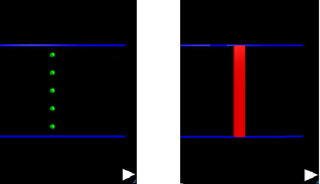
LHC-Neutrino fellow Jeremy Wegner wrote a program in VPython that does this online using the GlowScript platform. This has been simplfied for easy use. The setup is wth 5 target marbles as on the left but they are covered as on the right below:
A further description can be found in the introductory slides.
Here are the parameters for the current program file in GlowScript:
- URL of sim is http://cern.ch/go/Fp7l.
- Beam width (y) = 30 cm
- No. of targets = 5
- Radii of probes and targets are the same.
- Probes come from random values of y in x-direction, left to right.
- Each run has 10 trials (10 probe particles)
- Students cound number of probes bounced back to left after each run.
- To start a new run, choose the arrowhead at the bottom right.
- Each student does multiple runs, decided by teacher; total experiment should have at least 30 runs.
- Better - combine classes and schools to make large statistics.
- Watch this space for improvements.
One option for collecting the data is to use an online spreadsheet. Here is a Google sheet (view-only) that a teacher copy into his or her own Google drive:
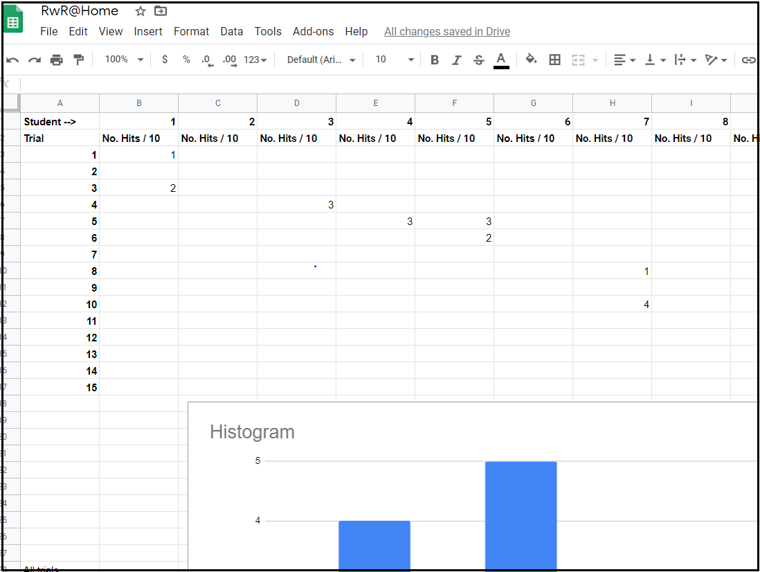
Once it is in your drive, you can make your copy editable to anyone with the link. Then each student can put results for up to 15 runs as it in now in their assigned column. (Students should not go into other columns and should only place numbers in their columns - no text.) There are a few numbers in the student columns already. These are placeholders and students should overwrite or delete them as they work.
Calculate the Z Mass
Comment:
Since our masterclass got interrupted by COVID and I wasn't able to do my usual suite of data activities at school as we were all sent home, I'm attempting to adapt the Z-mass activity for e-learning to hopefully give some insight into at least one of the particles my students are analyzing with the e-lab tools. I've split it up into 3 days to give students time to take each task one at a time and have the opportunity to ask questions and not get overwhelmed. For the first day I'm just having the students research information about the Z-particle and introduce them to the concept of E^2=p^2+m^2. I made a quiz on google classroom with relatively simple questions to answer that will hopefully guide their understanding of the situation. Second day is for measuring the vector info for the momentum of each muon and combining them; probably the toughest day with the most to do, but relatively little conceptual understanding necessary. And for the last day, after I've been able to review their results from the vector combination, they apply Einstein's equation to get the Z-mass. Relatively easy day, but with the most conceptual challenge. I'm just on the first day now, so no idea how it'll go; but also one way to adapt the data activities for e-learning.
Comment:
Overall I would say the activity adapted well to being done online. As anticipated, vector addition was the most difficult part for the students. This particular group of students really struggled with the concept of assigning an angle in a 360 degree system, but they did well using Einstein's equation to find the mass. Having each quarter on the event display divided into 10 parts makes a pretty good guess of the angle without a protractor relatively easy. It's a good introduction to particle concepts and is a good lead-in to discussing the peak at 90 GeV/c^2 on the IMC histogram. Discussions on conceptual understanding would probably have been more in-depth in a face-to-face setting, but in a pinch, I feel this worked pretty well; and I think as the students and I become more comfortable interacting online, they will ask more questions and I may find better ways to answer them more thouroughly.
Mean Lifetime Part 1: Dice
Comment:
A student can do this activity working remotely at home even if there are no dice available. The student can go to https://www.random.org/dice/ and set the number of dice to a number over, say 20. This is the procedure, using N0=40:
- Make a data table with the Number of Rolls in the left column and the Number of Dice Remaining in right column, This can be done on paper or in a spreadsheet. The first number in the Rolls column should be zero; each successive entry should be 1 greater, so the set in the Rolls column is {0,1.2.3.,,,}.
- Make the first number in the Dice Remaining column 40.
- On your computer, go to https://www.random.org/dice/.
- The site gives you a choice of how many virtual dice to roll. (The default is 2.) Set it to 40.
- Choose the "Roll Dice" button. A set of dice will appear.
- Count the number of dice with only one dot. Subtract this number from 40. Put this result in the second line of your table under Dice Remaining (just below 40), This will correspond to 1 under Rolls.
- On the site, choose the Go Back button.
- Change the number of virtual dice to the new number in your Dice Remaining column. (For example, this writer counted 7 one-dot dice and thus put 33 in the Dice Remaining column and then set the number of virtual dice to 33.)
- Choose the Roll Dice button.
- Count the number of one-dot dice.
- Subtract from your most recent Dice Remaining. Put this next in the same column.
- Choose the Go Back button.
- Change the number of virtual dice to the number you just added the new Number of Dice Remaining.
- Repeat steps 9-13 until you get to one die. Then stop and make a scatter plot.
Here is an example of a completed data table with plot:
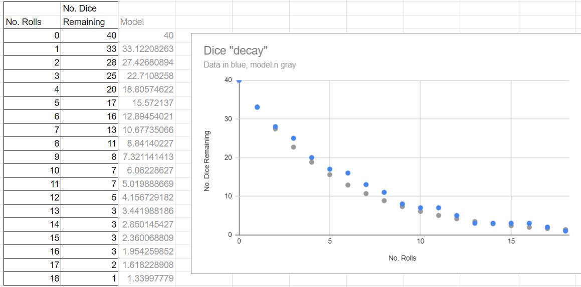
The extra column in gray is a calculation of the exponential decay model with a "lifetime" of 5.3 rolls. The blue dots in the plot show the data and the gray dots show the exponential decay fit.
Comment:
In the previous comment, we explained how to do this activity using an online dice simulator. Here, we use a little bit of (archaic) BASIC to do the same thing. The student would have to copy this program:
2000 CLS
2010 input "How many dice shall we roll?"; d
2020 if d=1 then goto 2200
2021 rem line 2020 makes nminumum no. dice = 1.
2030 print "You chose "; d; " dice."
2040 print
2050 for i=1 to d
2051 rem line 2050 starts loop, repeat d times
2060 let s = rnd(7)
2061 rem line 2060 gives a random number 0 to 5
2070 let q = int(s+1)
2071 rem line 2070 adds 1 and rounds down to an integer
2080 print q
2090 next i
2091 rem line 2090 closes the loop
2100 print
2110 for t=1 to 5000
2111 rem this is a delay loop
2120 next t
2130 input "What is your new number of dice? "; d
2140 for w=1 to 1000
2141 rem this is a delay loop
2150 next w
2160 goto 2020
2200 print
2210 print "The end."
It is available in this text file.
They can then paste it into an online BASIC tool like http://www.quitebasic.com/. Students can start with an intial number of dice, subtract the number of 1's they get, and then input the new number of dice. Students need to fill out their number of data tables as they go.
Having the program also allows students to modify it to see what they can do with this old but workable programming language.
What Heisenberg Knew
No comment: can be used as is for remote learning.
Histograms: Uncertainty
Comment:
This activity lends itself well to remote learning with a few adaptations.
Part I needs no adaptation: what is in the Student Guide will suffice.
For Part II, the student needs either a printer, a computer with a drawing program like MS Paint, or internet access to on online drawing program like jspaint. The student must either print out the Figure 2 from the Student Guide or open on a computer. If it is printed out, the student can calculate and then draw in the error bars. If using a Paint, jspaint, or somenthing similar, they can open the plot image and then draw in the error bars as thick lines. This writer used red in jspaint on the first two bars of the graph to show how it can be done:
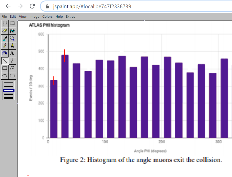
For Part III, students need, again, to either print out and draw on Figure 4 from the Student Guide or work with it digitally as described for Part II.
Energy, Momentum, and Mass
No comment: can be used as is for remote learning.
CMS Data Express
No comment: can be used as is for remote learning.
Mean Lifetime Part 2: Cosmic Muons
No comment: can be used as is for remote learning.
ATLAS Data Express
No comment: can be used as is for remote learning.
Making it 'Round the Bend - Quantitative
Comment:
Students can do this activity at home provided they have computers wwhich can download, uncompress, and run the simulations.
Mean Lifetime Part 3: MINERvA
No comment: can be used as is for remote learning.
Cosmic Ray e-Lab
No comment: can be used as is for remote learning.
CMS Ray e-Lab
No comment: can be used as is for remote learning.